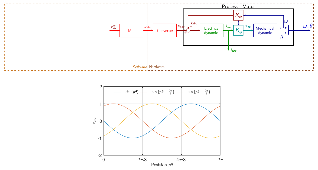
where \(i_{abc} = \left[\begin{matrix}i_a & i_b & i_c\end{matrix}\right]^\intercal\) are the stator phase currents, \(v_{abc} = \left[\begin{matrix}v_a & v_b & v_c\end{matrix}\right]^\intercal\) the stator phase voltages, \(\Omega\) and \(\theta\) are the speed and position respectively and \(p\) the pole pair number. \(L\) and \(R\) and the staotr inductance and resistor, \(\phi_f\) the flux constant. \(\tau_r\) the resistive torque and \(\tau_m\) the motor torque.
\[\begin{equation} \tau_m = -p\phi_f \left[i_a\sin(p\theta) + i_b\sin\left(p\theta-\frac{2\pi}{3}\right) + i_c\sin\left(p\theta+\frac{2\pi}{3}\right)\right] \end{equation}\]
Clarke-Parc Transformations
Under the assumption of balanced motor one has \(x_a+x_b+x_c = 0\). Motor equations can thus be transformed into a 2-phases equivalent representation using Clarke transformation.
\[\begin{equation} x_{\alpha\beta} = \begin{bmatrix}x_\alpha & x_\beta\end{bmatrix}^\intercal = T_{3\rightarrow2}x_{abc} = T_{3\rightarrow2}\begin{bmatrix}x_a & x_b &x_c\end{bmatrix}^\intercal \end{equation}\] \[\begin{equation} T_{3\rightarrow2} = \frac{2}{3}\begin{bmatrix}1 & -\frac{1}{2}& -\frac{1}{2}\\0 & \frac{\sqrt{3}}{2}& -\frac{\sqrt{3}}{2}\end{bmatrix} \end{equation}\] \[\begin{equation} \label{eq:modeleab} \left\{\begin{array}{rcl} L \frac{di_{\alpha}}{dt} & = & v_{\alpha}-R i_{\alpha}+ p \phi_f \Omega \sin(p\theta)\\\\ L \frac{di_{\beta}}{dt} & = & v_{\beta}-R i_{\alpha}- p \phi_f \Omega \cos\left(p\theta\right)\\\\ J\frac{d\Omega}{dt} &=& \tau_m -\tau_r \\\\ {\frac{d\theta}{dt}} &=& \Omega\\ \end{array}\right. \end{equation}\] \[\begin{equation} \tau_m = p\frac{3}{2}\phi_f \left[-i_\alpha\sin(p\theta) + i_\beta\cos(p\theta)\right] \end{equation}\]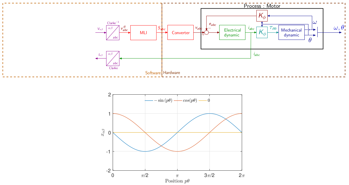
In the previous model, votages and currents varies at high frequency (p times the rotational frequency). To avoid sinus terms Park transformation is used (Par29).
The Park transform is a rotation matrix \(R(\theta)\) from \(\alpha\beta\) axes to \(dq\) axes. One as
\[\begin{equation} \label{eq:park} x_{dq} = R(\theta) x_{\alpha\beta} = \left[ \begin{matrix} \cos(p\theta) & \sin(p\theta)\\ -\sin(p\theta) & \cos(p\theta) \end{matrix} \right]x_{\alpha\beta} \end{equation}\] \[\begin{equation} \label{eq:invpark} x_{\alpha\beta} = R(\theta)^{-1} x_{dq} =\left[ \begin{matrix} \cos(p\theta) & -\sin(p\theta)\\ \sin(p\theta) & \cos(p\theta) \end{matrix} \right]x_{dq} \end{equation}\]The model in the \(dq\) frame is :
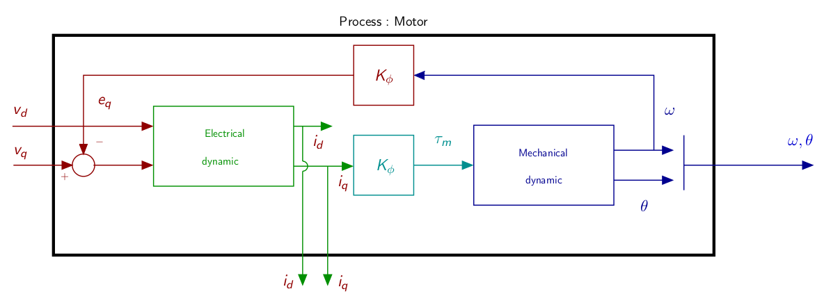
\[\begin{equation} \label{eq:modeledq} \left\{\begin{array}{rcl} L \frac{di_d}{dt} & = & v_d-R i_d + Lp\Omega i_q\\\\ L \frac{di_q}{dt} & = & v_q-R i_q - Lp\Omega i_d -\phi_f p\Omega\\\\ J\frac{d\Omega}{dt} &=& \tau_m -\tau_r \\\\ {\frac{d\theta}{dt}} &=& \Omega\\ \end{array}\right. \end{equation}\] \[\begin{equation} \tau_m = p\frac{3}{2}\phi_f i_q \end{equation}\]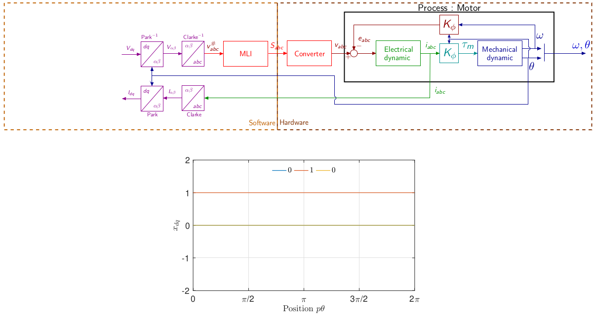
(Par29) Park, R.-H. (1929). Two-reaction theory of synchronous machines generalized method of analysis-part I. Transactions of the American Institute of Electrical Engineers, 48(3), 716–727. https://doi.org/10.1109/T-AIEE.1929.5055275